Deconvolution and Noise Reduction Example with M81 and M82
Processing example by Juan Conejero (PTeam)
With original data acquired by Harry Page
Introduction
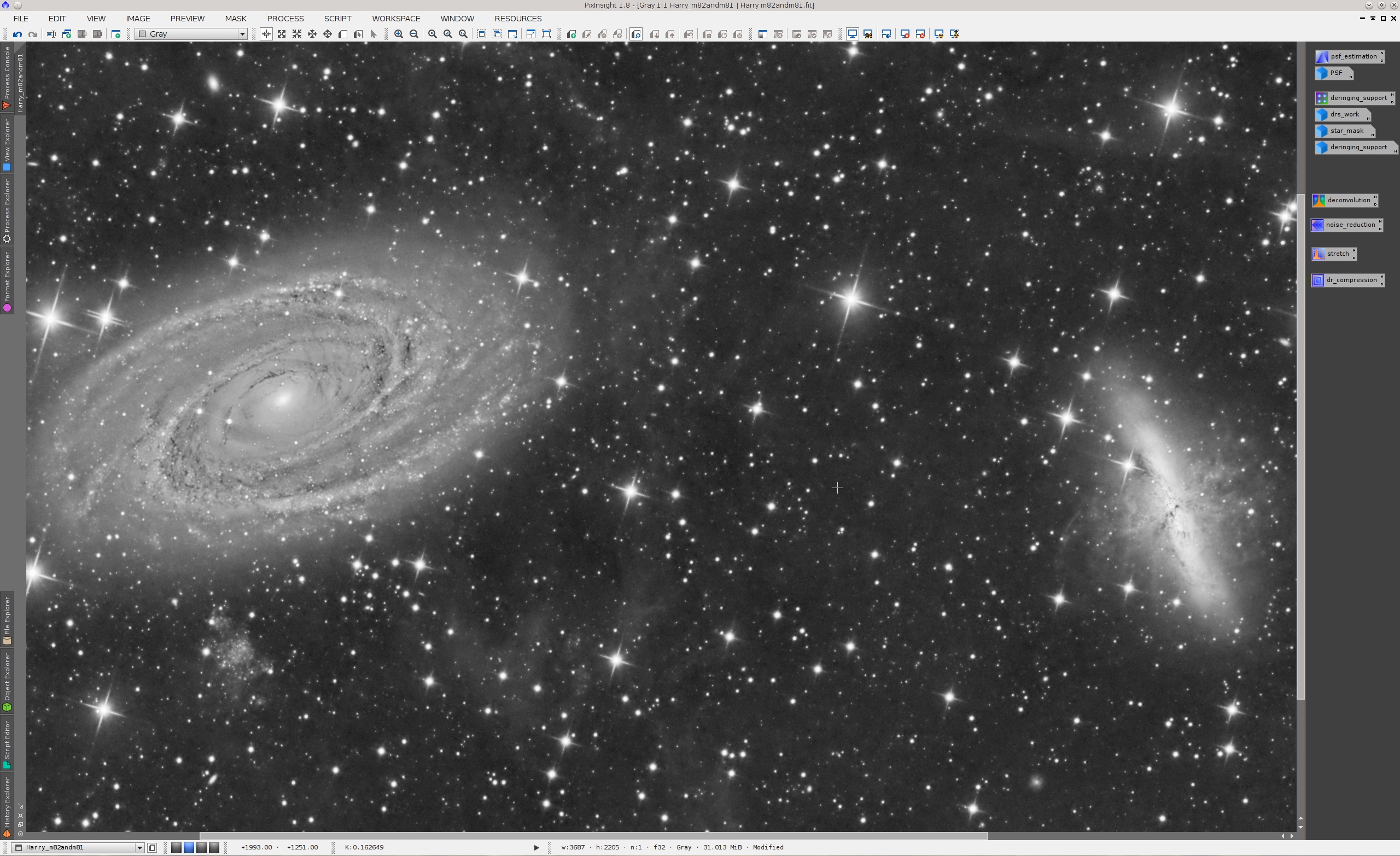
Back in June of 2011 I wrote a noise reduction tutorial with a nice image of the M81 and M82 region by Harry Page. Since then we have released new tools and improved versions of already existing tools, which deserve up-to-date information and processing examples.
So here is a new tutorial that I have just written with the same image. To put noise reduction in a more practical context, this time I'll develop a more complete example including deconvolution, noise reduction in the linear stage, nonlinear stretching, and dynamic range compression. Thanks again to Harry Page for letting me use these excellent data.
I hope you'll find this tutorial useful to understand and apply several key image processing techniques and tools. At the risk of stating the obvious, tutorials like this one are not step-by-step instructions that can be followed literally, or applied to process any similar image without the necessary analysis. Use it to learn the concepts described, but keep in mind that each image poses different problems and requires you to devise your own solutions creatively.
Fitting a PSF Model
Since we are going to apply deconvolution, our first step is to get an accurate model of the point spread function (PSF) of the image. The following screenshot shows the DynamicPSF tool with 60 fitted stars. Of course the image is linear—a PSF fitting process and the subsequent deconvolution would make no sense at all otherwise—, so it is visible thanks to the ScreenTransferFunction tool and its AutoStretch routine.
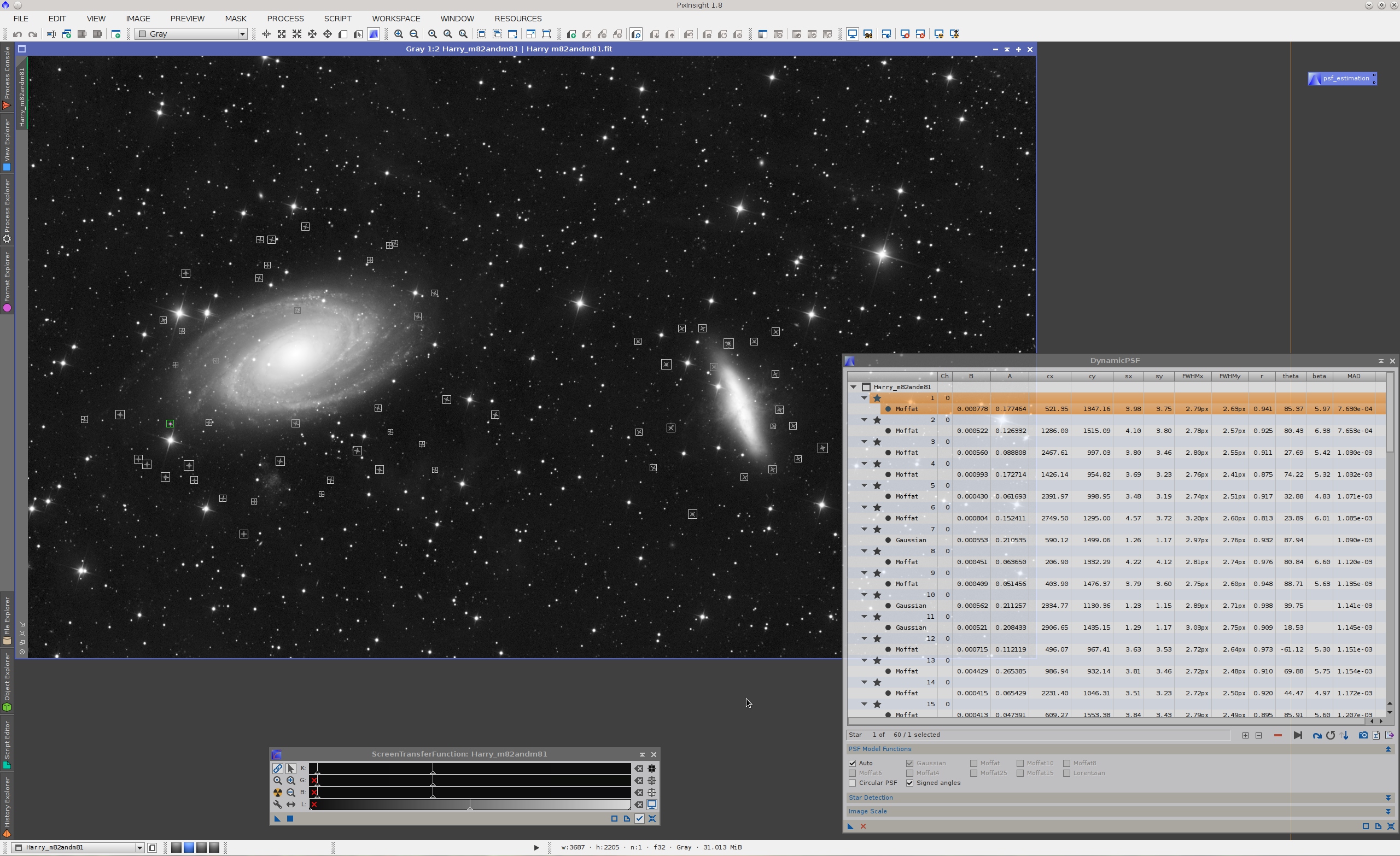
After fitting some 60 stars around the main subjects of the image, I have sorted the list by increasing order of MAD (median absolute deviation, used here as a goodness-of-fit estimate), and have generated a robust PSF model from the 50 best stars with DynamicPSF's Export synthetic PSF option.
Building a Local Deringing Support
The Gibbs phenomenon is the mathematical explanation of the ringing artifacts that linear high-pass filtering procedures generate around jump discontinuities such as stars, planetary limbs and, in general, around any high-contrast edge or small-scale image structure. Ringing is a very difficult problem that limits the applicability of most restoration algorithms to real-world images.
Our solution to the ringing problem in our current Deconvolution tool is twofold. On one hand we implement a global deringing algorithm that acts on the whole image after deconvolution, recovering ringing artifacts with original pixels partially like a sort of localized flat fielding process. We implement also a local deringing regularization algorithm that works at each deconvolution iteration limiting growth of ringing artifacts. This local deringing is driven by a local deringing support image, where nonzero pixels define the amount of deringing regularization applied.
So the next step toward deconvolution is building a local deringing support. As I have pointed out many times, a deringing support is not a mask, although in the case of a deep-sky image, it looks like and is built essentially as a star mask. There are many ways to generate star masks in PixInsight. In this case I'll put an example of the most obvious option: the StarMask tool. However, to help StarMask achieve an optimal result more quickly, it is generally convenient to pre-process the image to facilitate isolation of stars and other small-scale, high-contrast structures. Again, there are several methods to perform this step. On a duplicate of the image, I have removed the first and residual wavelet layers in a five-layer decomposition, as shown on the next screenshot.

To this image we can apply the StarMask tool with the following result:
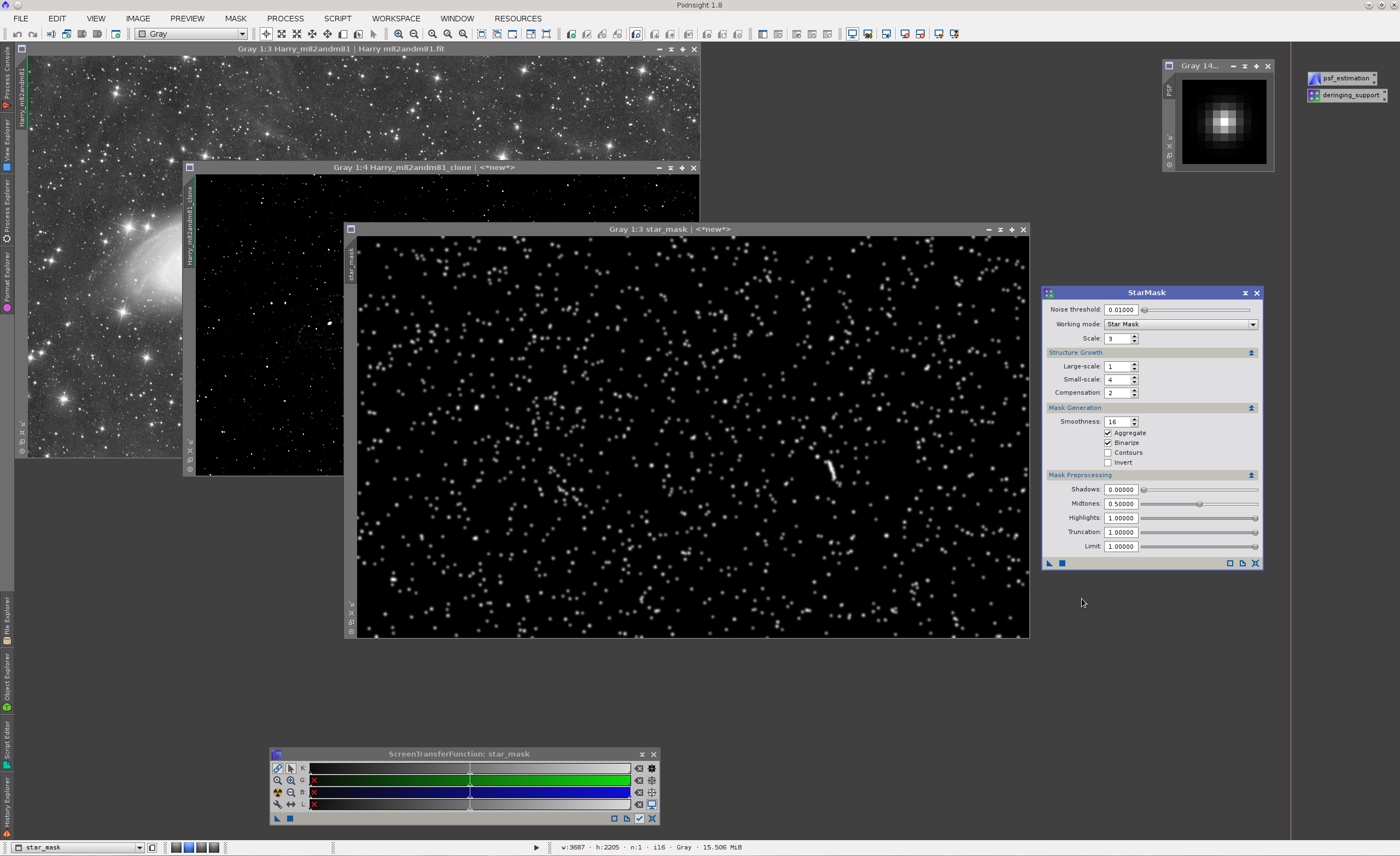
On the screenshot above, note that I have altered a number of StarMask parameters:
- Noise threshold has been decreased to include the necessary structures in the generated mask. After preprocessing with the starlet transform the image has virtually no noise, so we can use this parameter effectively to control inclusion of dim stars in the mask.
- Scale has been decreased to prevent inclusion of large-scale residuals left after suppression of wavelet layers, such as traces of the spiral arms of M81, and some traces of the core of M82.
- Large-scale growth has been decreased to prevent excessive dilation of bright stars. We need to cover the regions where ringing can be problematic, but not more.
- Small-scale growth has been increased to improve protection around mid-sized stars.
- The aggregate option has been enabled. This tends to produce masks more proportional to the actual brightness of original image structures.
- The binarize option has been enabled in this case to generate a stronger mask.
In general, local deringing support images only need to include relatively large stars, since global deringing is already quite efficient to fix ringing around most structures. This image is a rather difficult case, especially because of some stars projected on the central areas of M81 and M82, where ringing artifacts may easily become objectionable. Always keep in mind that deringing tends to degrade the deconvolution process, so one must find the required dose for each particular image. Also take into account that a very small amount of visible ringing can be beneficial rather than harmful, since it increases acutance, which in turn favors the visual perception of detail.
Our mask includes now the stars that may require special protection, but it also includes some unwanted structures. As you can see, some nonstellar image features have been gathered by the mask over M82. This happens because, as seen by the applied multiscale analysis, these structures are similar to stars. If we leave these structures in the mask, they will degrade deconvolution precisely where we want it to reveal many hidden details in M82, which is not what we want.
A quick and dirty but effective way to solve this problem would be applying CloneStamp, or a similar painting tool, to manually remove the unwanted mask structures. Since bright stars can be understood as singularities in this case—that is, as objects where the algorithms that we are going to use cannot be applied—, I don't see any problem in doing this to overcome a limitation of the multiscale analysis techniques that we have used to generate the star mask, from a documentary point of view.
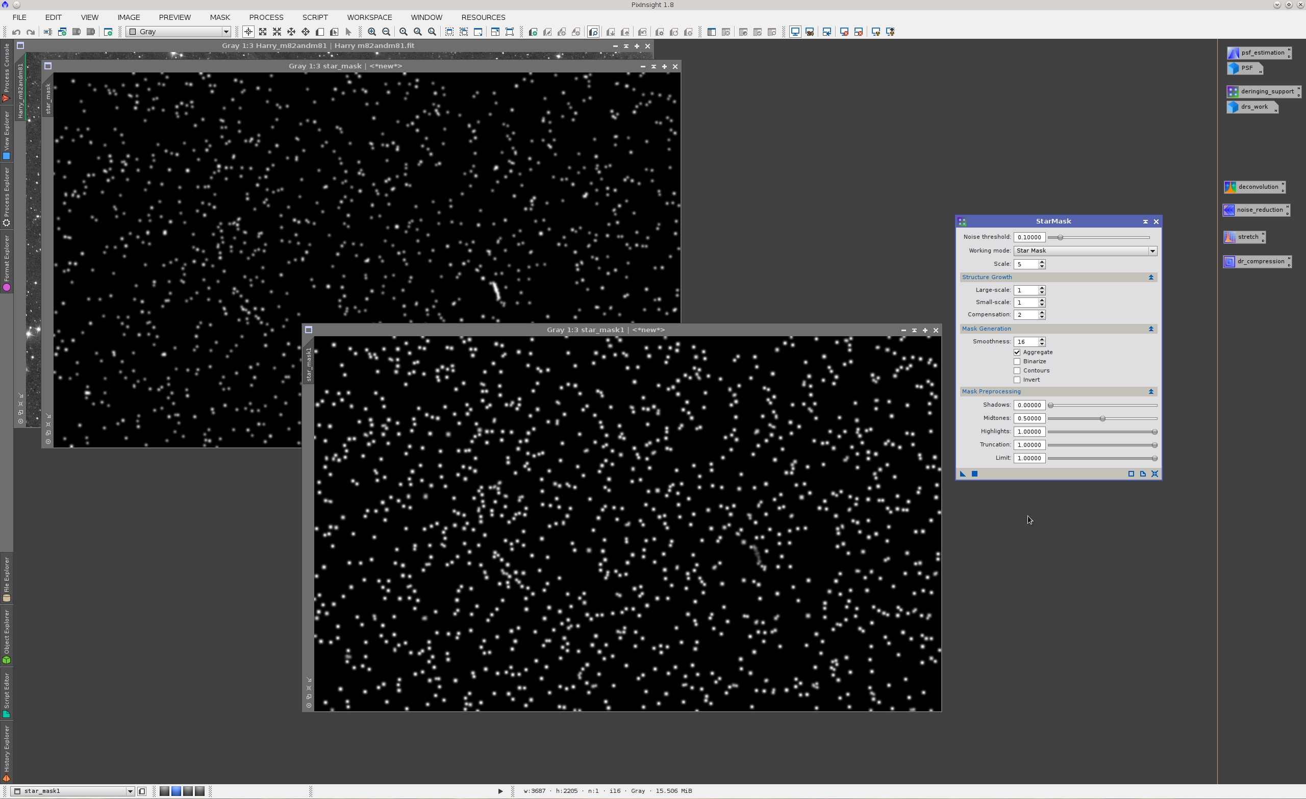
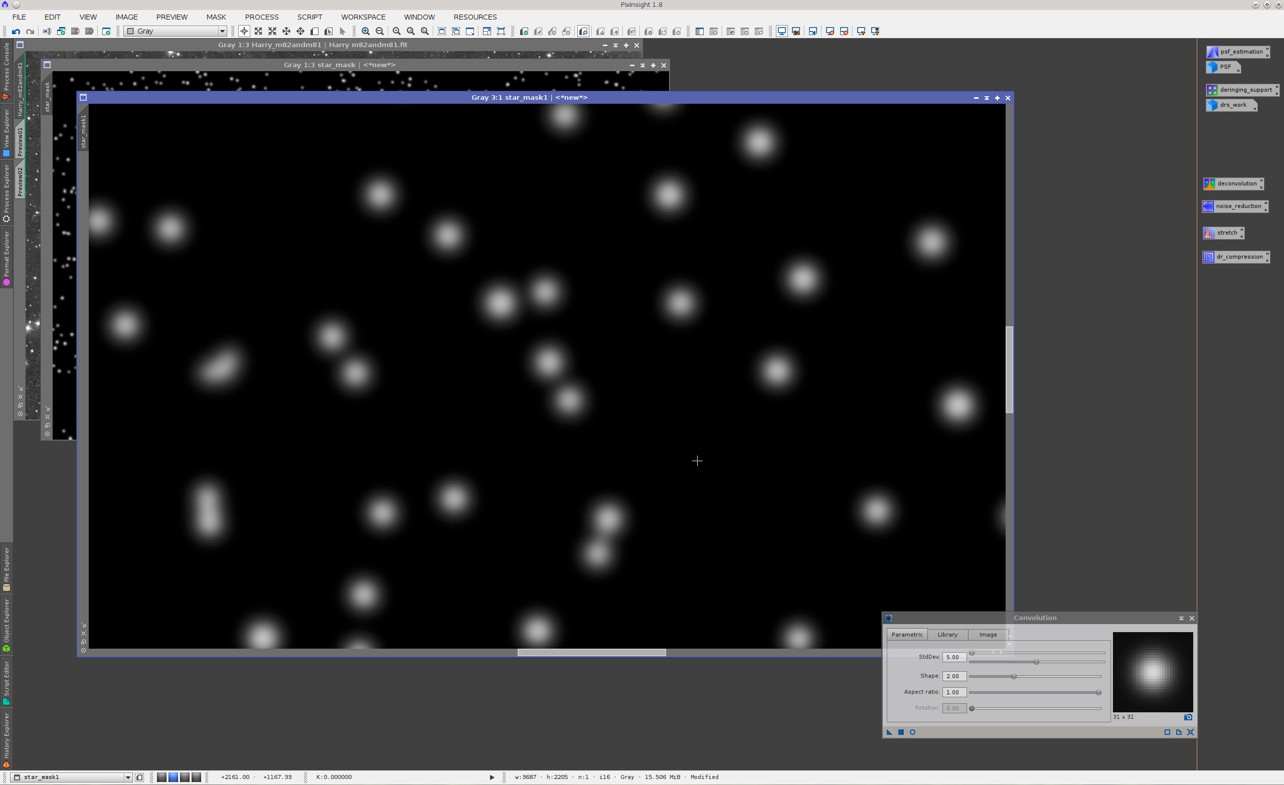
But since we are here to offer more creative solutions, I'll describe a way to exclude the unwanted structures using pure image processing resources, without manual intervention. If we apply a new instance of StarMask to the star mask, we can refine isolation of mask structures within a typical range of interest. In the case of this image, if we limit structure detection to the first five wavelet layers, the structures on M82 are strongly diminished in the resulting mask. This happens because the morphology and size of these structures become "atypical" in the mask under this new analysis:
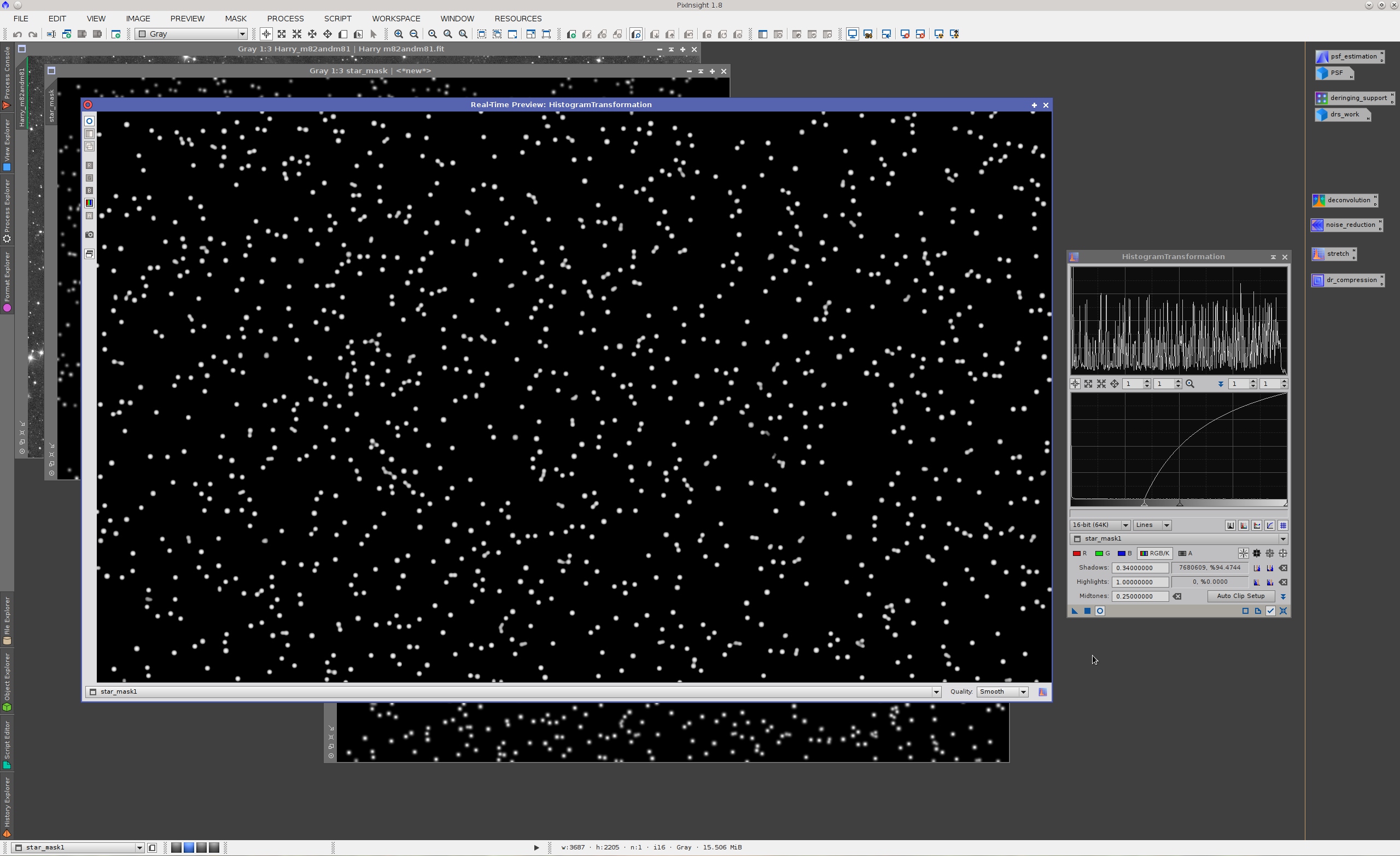
A simple histogram clip allows us to get rid of most of these residuals very easily:
And finally, a convolution with a Gaussian filter allows us to control the smoothness of mask edges:
Deconvolution
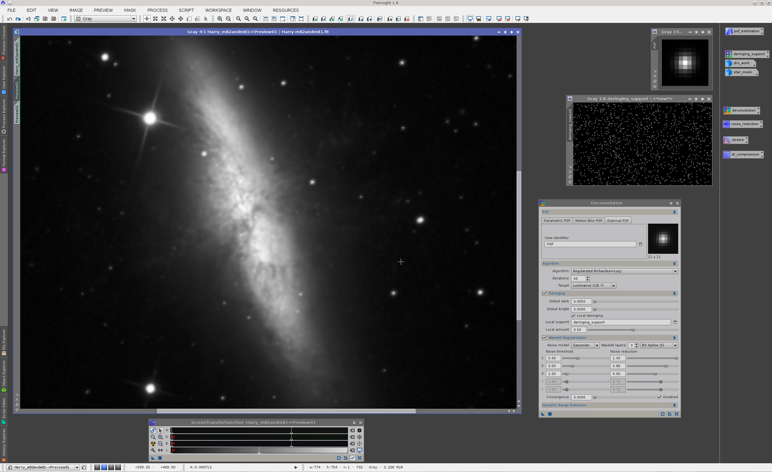
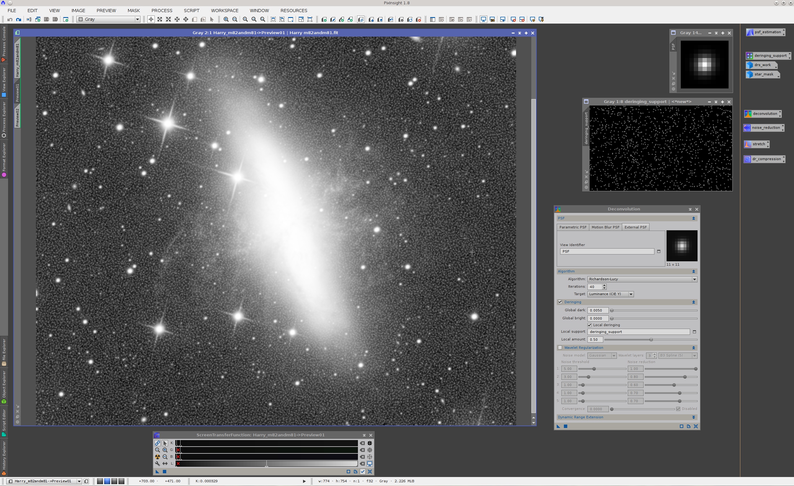
After renaming the modified star mask image to "deringing_support" for easy identification, this is our setup for deconvolution:

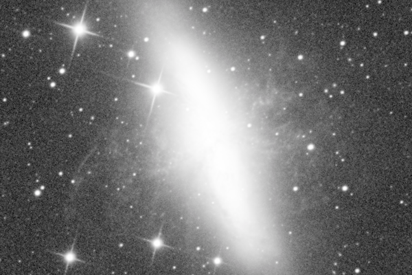
I have selected a preview on M82 to test deconvolution parameters. Note that I have used custom STF settings to reveal the central regions of the galaxy. This is the same preview after deconvolution:
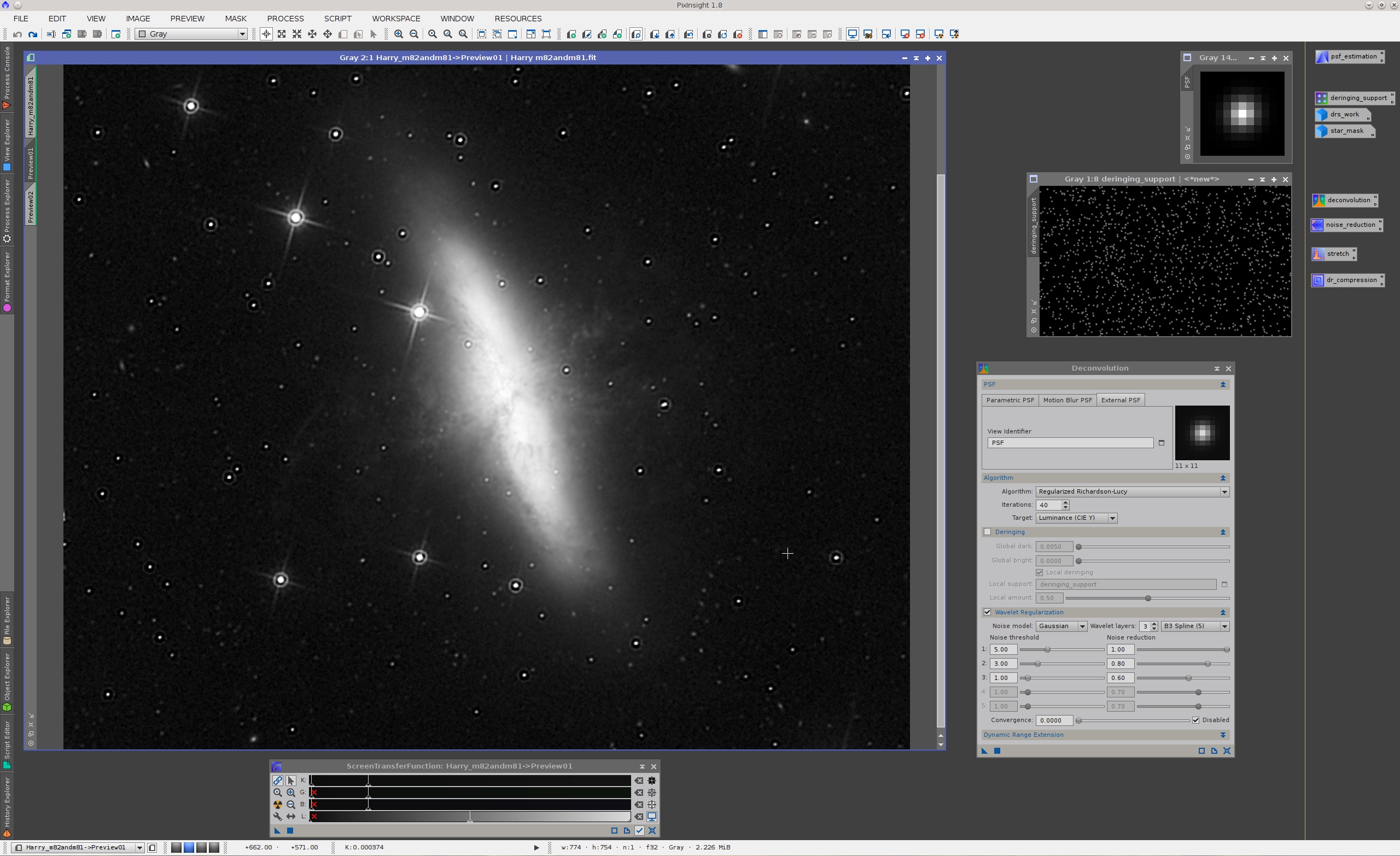
One must always be careful to test the results of deconvolution thoroughly, including different STF parameters to evaluate not only the quality of image restoration for significant structures, but also the efficiency of regularization on background or low-signal regions. This is the preview with automatic screen stretch parameters before deconvolution:

and after deconvolution:

The following deconvolution parameters deserve some pointing out:
- We are using an external PSF image, which is the PSF estimate that we have computed with the DynamicPSF tool at the beginning of this tutorial.
- The regularized Richardson-Lucy algorithm [4][5] usually yields the best results for deconvolution of deep-sky images.
- Generally between 20 and 50 iterations are sufficient to achieve a good result.
- In this example we are using both the global and local deringing algorithms, the latter with the deringing support image that we have constructed in the preceding section. For many images global deringing is sufficient. It depends on the difficulties posed by bright stars, especially when they lie over relatively bright surfaces. From my experience, this image can be considered as a moderately difficult case.
- The local amount deringing parameter can be used to fine tune the amount of local deringing applied. This parameter is just a multiplying factor for the local deringing support.
- Wavelet regularization must be fine tuned to prevent noise intensification on low-signal areas. As happens with deringing (which can be understood as a special type of regularization), the less is the better: one must find the smallest amount of regularization that cancels noise intensification, since excessive regularization may damage significant image structures.
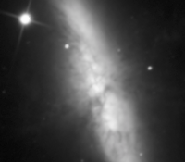
Mouse over:
Before deconvolution
After deconvolution
Figure 1— Before/after comparison of deconvolution, image enlarged 3:1.
One of the best ways to understand how the different deconvolution parameters work is by comparing the same image processed with and without them. Let's begin with the result of deconvolution without deringing:
Now with global deringing only, hence with no local deringing:

And this is without regularization:
It is worth mentioning that we have used no protection mask to apply deconvolution. A mask can be used to protect low-signal areas such as the sky background and faint structures, but with the wavelet regularization algorithms that we have implemented in our tool a protection mask is optional, as I have just demonstrated in this example.
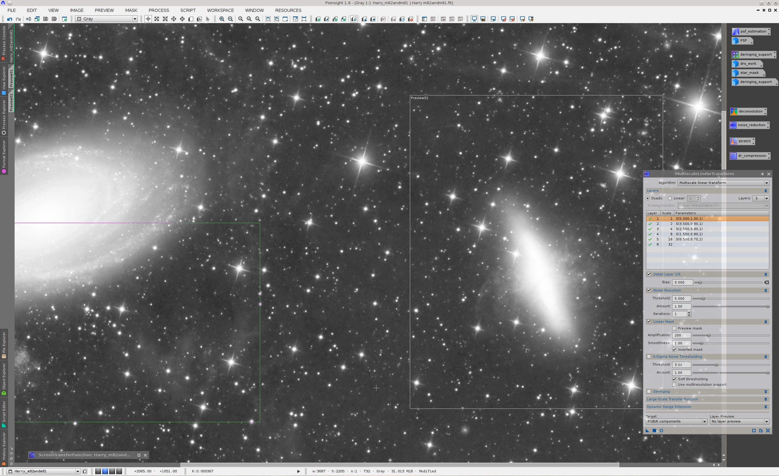
Noise Reduction
In the latest versions of PixInsight we have implemented two new multiscale analysis algorithms: the multiscale linear transform (MLT) as an alternative to the starlet wavelet transform [1][2] (SWT, also known as à trous wavelet transform or ATWT), and the median-wavelet transform (MWT) [2][3] as a complement to the multiscale median transform (MMT). [2][3] In this example I'll use MLT, which has proven to be very efficient and controllable for noise reduction of linear deep-sky images. The MWT algorithm could also be used with similar results.
Irrespective of the algorithm used, our multiscale analysis tools also include a linear mask feature. The idea is pretty simple: for noise reduction of linear deep-sky images, the strength of noise reduction should always be a function of the noise-to-signal ratio. A linear mask is a very efficient data structure to achieve that goal. It is a duplicate of the image transformed only by linear operations: a multiplicative factor that we call amplification, a signal clipping based on robust statistics (which acts internally in an automatic way), and a convolution for edge softening purposes, which we control with the smoothness parameter. The linear mask feature has a preview option that can be used to facilitate the search of good mask generation parameters:
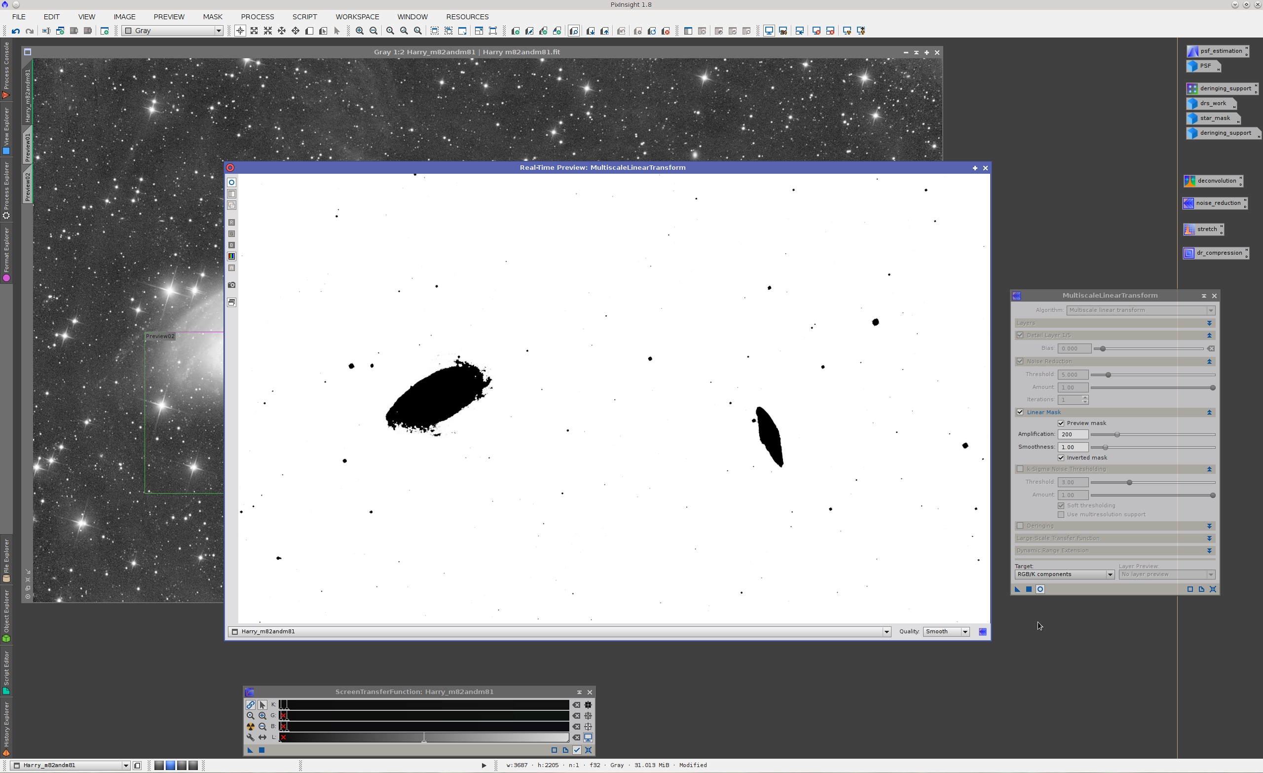
Obviously the mask must be inverted for noise reduction, since it should protect bright regions. An additional mask inversion option allows applying these tools to inverted images with dark objects over bright backgrounds.
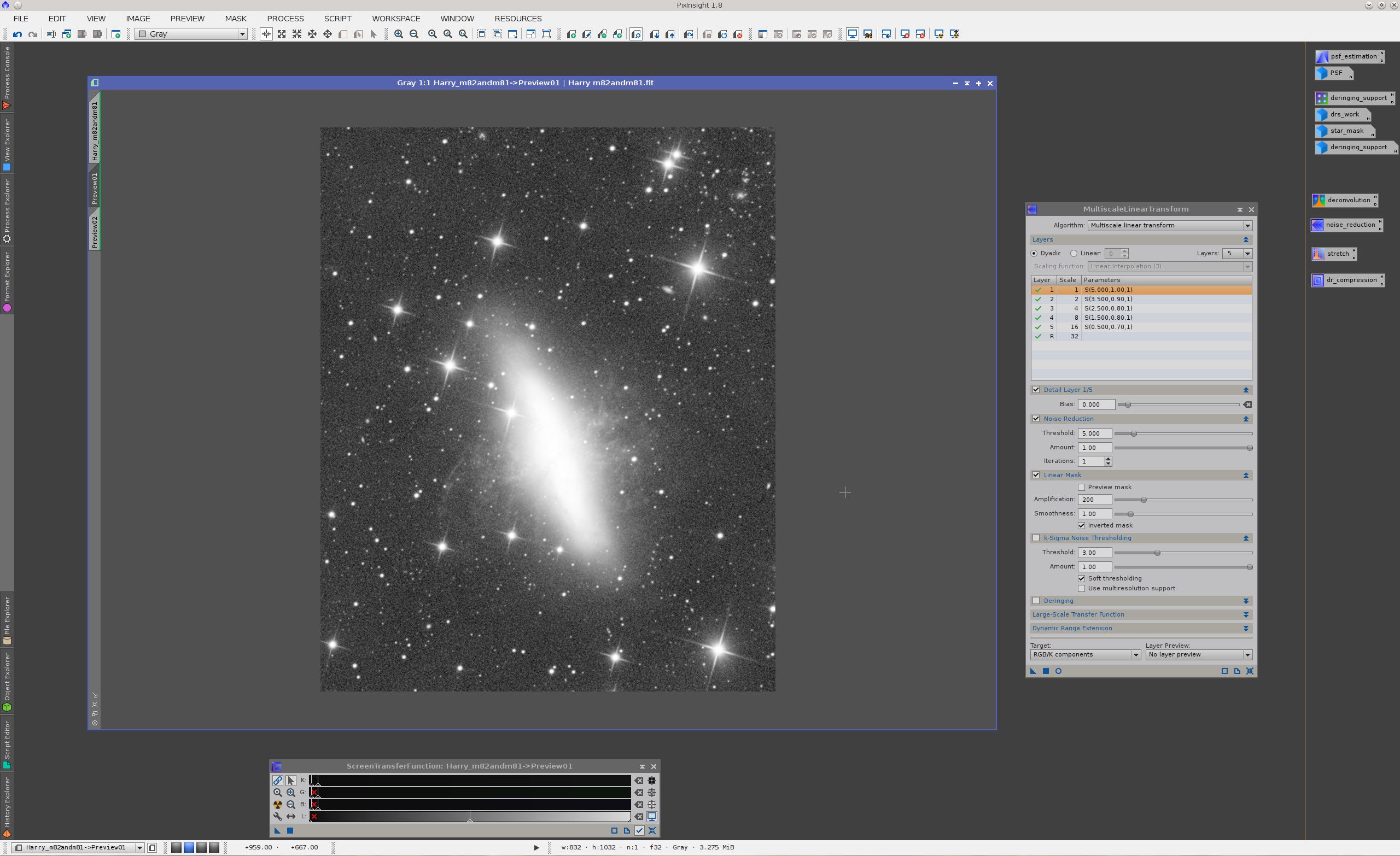
Once we have found good linear mask parameters—which is much easier than what may seem at first sight, since the tool guides the process—we can try out the MLT algorithm. This is before noise reduction:
And after noise reduction with MLT:

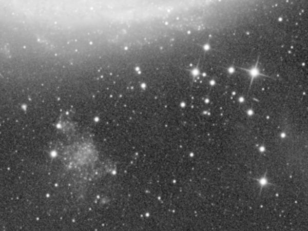
The same comparison on a preview covering part of M81 and some nice integrated flux nebulae (IFN):
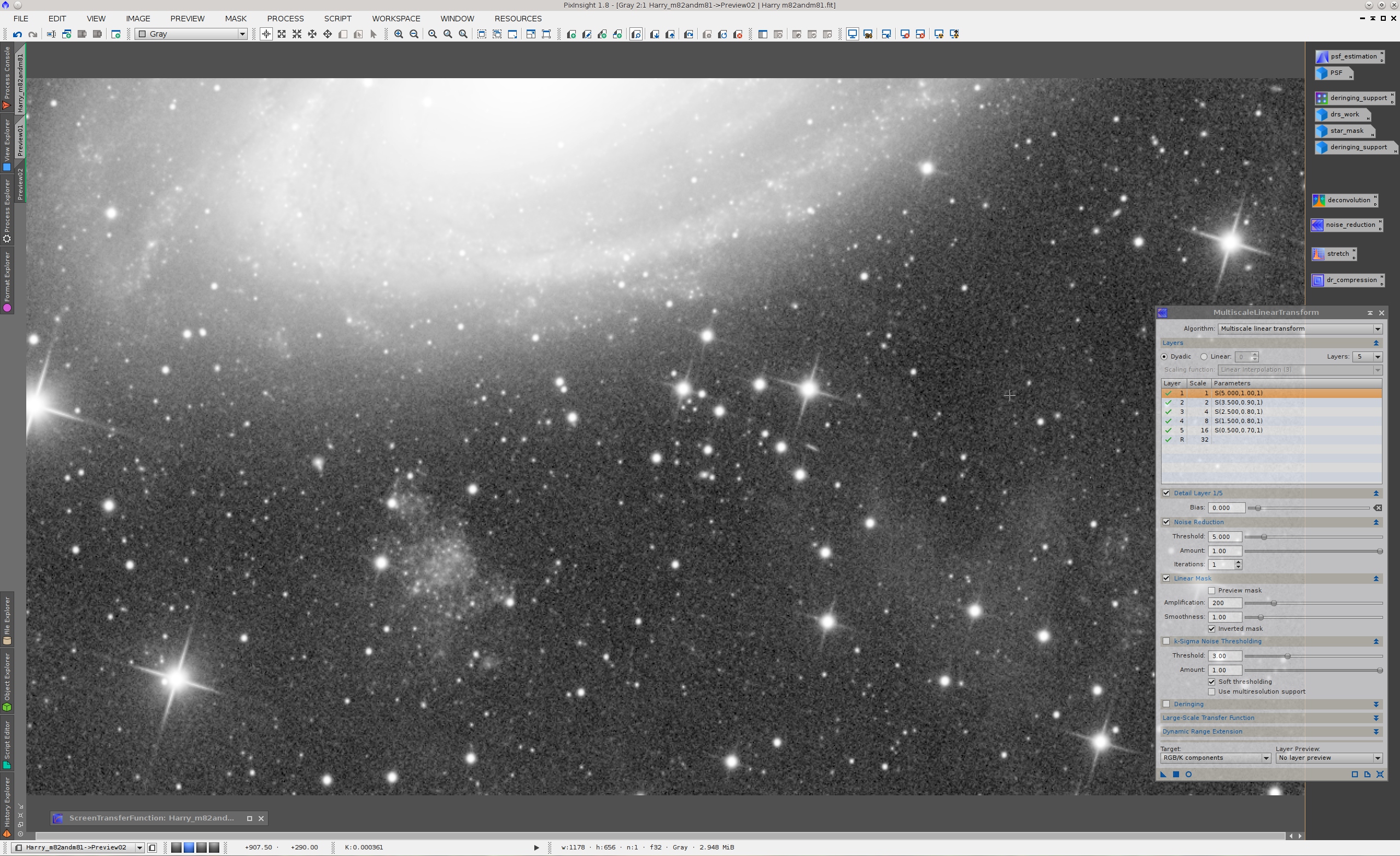

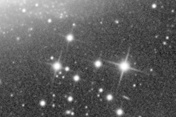
The goal of any noise reduction procedure is to achieve a sufficient noise reduction while significant structures are preserved. Here is a view of the denoised image at its actual size:
A mistake that we see too often these days is trying to get an extremely smooth background without the required data support. This usually leads to "plastic looking" images, background "blobs", incongruent or unbelievable results, and similar artifacts. Paraphrasing one of our reference books,[6] this is like trying to substantiate a questionable hypothesis with marginal data. Observational data are uncertain by nature—that is why they have noise, and why we need noise reduction—, so please don't try to sell the idea that your data are pristine. We can only reduce or dissimulate the noise up to certain limits, but trying to remove it completely is a conceptual error: If you want less noise in your images, then what you need is to gather more signal.
Mouse over:
Before noise reduction
After noise reduction
Figure 2— Before/after comparison of noise reduction, actual image size.
Mouse over:
Before noise reduction
After noise reduction
Figure 3— Before/after comparison of noise reduction, actual image size.
Mouse over:
Before noise reduction
After noise reduction
Figure 4— Before/after comparison of noise reduction, image enlarged 2:1.
The following MLT parameters are worth noting in this example:
- Noise reduction has been applied to five multiscale layers following a dyadic decomposition scheme, that is to scales of one, two, four, eight and sixteen pixels. Except for images with very little noise, generally the noise cannot be isolated only in the first small-scale layers. Some analysis algorithms are more efficient at isolating structures, such as the multiscale median transform compared to linear transforms such as starlet or MLT.
- The amount noise reduction parameter of our multiscale analysis tools allows you to fine tune the degree of noise reduction applied at different dimensional scales. Remember that trying to suppress the noise completely is an excellent way to destroy your data.
- The threshold noise reduction parameter controls the amount of transform coefficients removed or attenuated on each layer. Thresholds are expressed in sigma units, or units of the statistical dispersion or variability of transform coefficients. In general, the smallest coefficients (in absolute value) are due to the noise, while larger coefficients tend to support significant image structures. Higher thresholds are more inclusive, so they tend to reduce more noise; however, too large of a noise reduction threshold can damage significant structures. Typical thresholds for the first layer of MLT or SWT are between 3 and 5 sigma. Successive layers usually require smaller thresholds, as you can see in the screenshots of this tutorial. Always be very careful to prevent artifacts caused by excessive noise reduction. Try out your parameters thoroughly on different previews covering relevant areas of the image.
- The iterations parameter, which I haven't used in this example, can be useful to get more control on the noise reduction process, especially in combination with values of the amount parameter between 0.5 and 0.7. It can also be used to apply a stronger noise reduction, when necessary.
Nonlinear Stretch
After noise reduction we have finished processing the image in its linear state, so our next step is to apply a nonlinear transformation commonly known as initial stretch. The purpose of this initial stretch is to adapt the image to our visual system, which has a strongly nonlinear response, as well as to make it directly representable on output devices that emulate our visual response, such as monitors and other display media.
The initial stretch is one of the crucial processes that determine the very final result. If wrongly implemented, you can easily destroy your data, raise it to unrealistic levels, or simply fail to show it as it deserves. Again, this process can be implemented in different ways in PixInsight. The most common tool for this purpose is HistogramTransformation, which I have used in this tutorial.
On the above screenshot, note how I have clipped a small unused section of the histogram at the shadows. This unused segment is a typical and nice result of noise reduction. This operation must always be done very carefully to avoid clipping significant data. In this case I have clipped just five pixels.
For deep sky images like this one, the main peak of the histogram—which identifies the average background of the image—should not be set to a too low value. I usually set it around 0.12 or 0.15, leaving an unused gap at the left side when necessary. Deep sky astrophotography is all about the dim stuff, which needs a relatively bright background to become well visible.
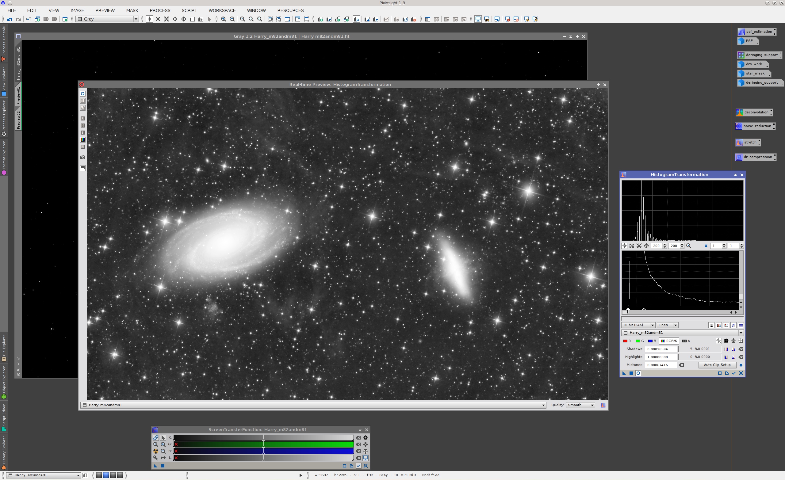
Dynamic Range Compression
Large and bright regions of many deep sky objects tend to hide smaller structures on well exposed images. This happens frequently with galaxies and bright nebulae, being M42 and M31 two well-known paradigmatic cases. When this happens, we say that we have a dynamic range problem. Note that this includes but is not limited to multi-exposure high dynamic range images. On single-exposure deep-sky images we often have to face serious dynamic range problems, as pose the two galaxies in the image of this tutorial. Are the cores of M81 and M82 really burned out as they look like on the above screenshots after the initial stretch? Actually, they are not only not burned at all, but are hiding an impressive amount of detailed image features that claim to be unveiled.
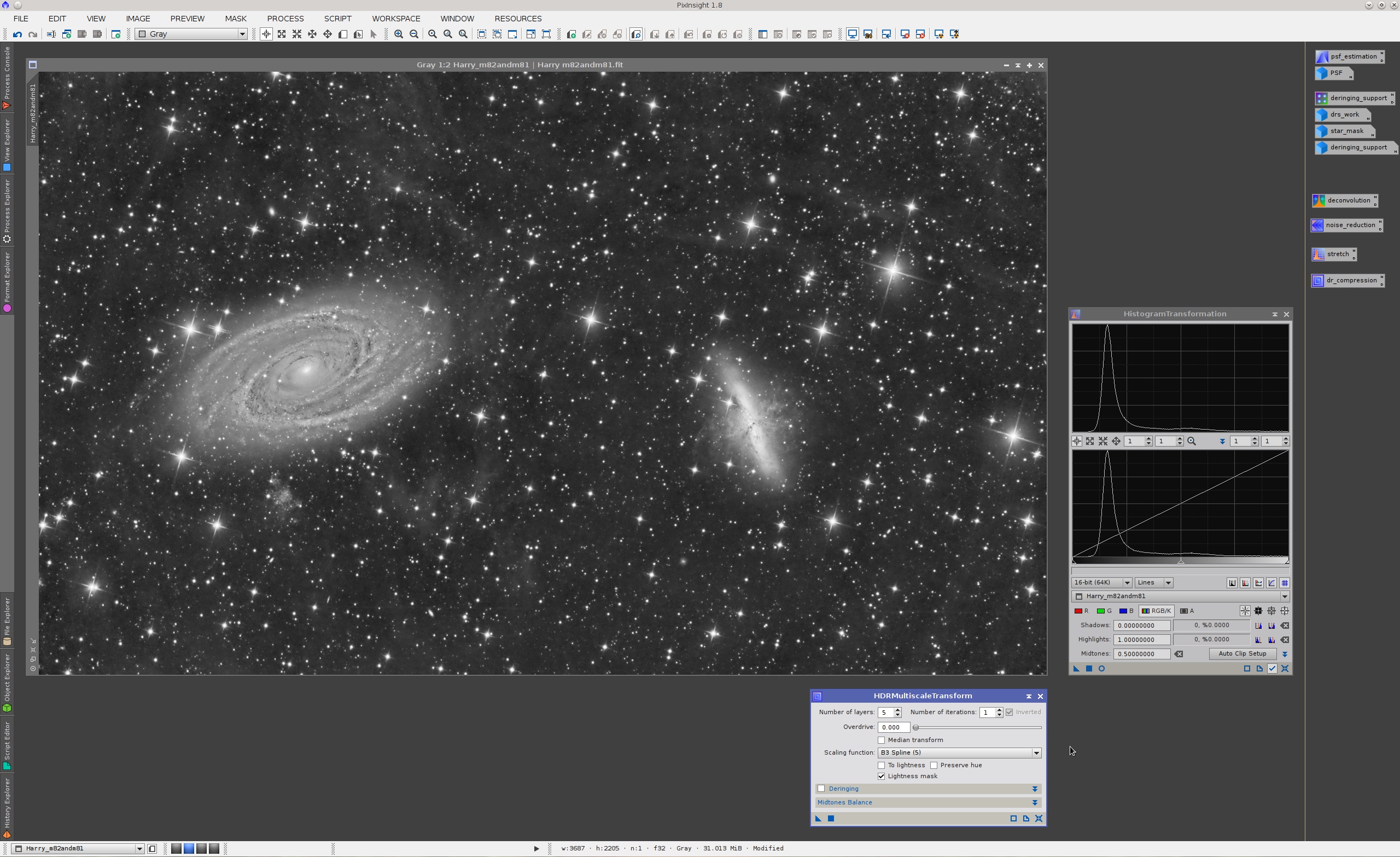
We have a good bunch of dynamic range compression tools and procedures implemented in PixInsight. Our most famous and powerful tool for dynamic range management is HDRMultiscaleTransform (HDRMT). This tool implements an algorithm created by PTeam member Vicent Peris in 2006, which we have been further developing and improving at a constant rate during the last years.
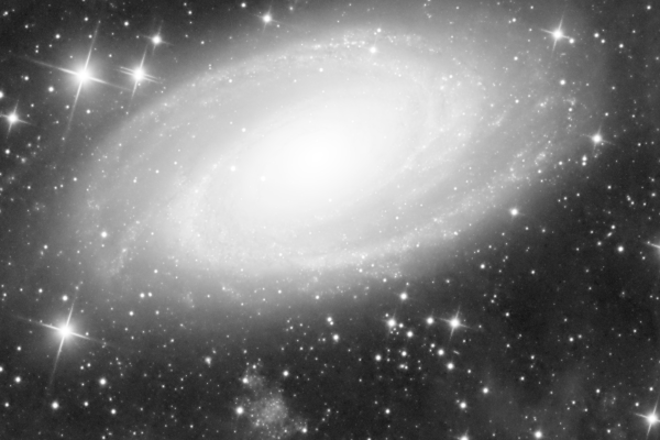
Mouse over:
Before dynamic range compression
After dynamic range compression
Figure 5— Before/after comparison of dynamic range compression, image zoomed out 1:2.
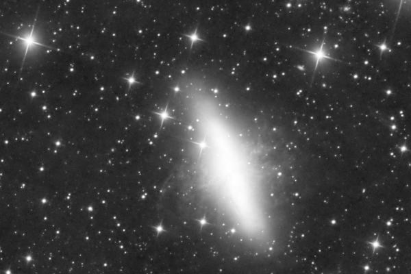
Mouse over:
Before dynamic range compression
After dynamic range compression
Figure 5— Before/after comparison of dynamic range compression, image zoomed out 1:2.
As you see, the result after HDRMT is simply amazing. Now we have a final product that really makes justice to the original data. After dynamic range compression, the documentary value of the image has increased exponentially, to the point that now it is a vehicle to communicate the true nature and structure of these wonderful galaxies:
References
[1] Jean-Luc Starck, Fionn Murtagh, Mario Bertero (2011), Handbook of Mathematical Methods in Imaging, ch. 34, Starlet Transform in Astronomical Data Processing, Springer, pp. 1489-1531.
[2] Starck, J.-L., Murtagh, F. and J. Fadili, A. (2010), Sparse Image and Signal Processing: Wavelets, Curvelets, Morphological Diversity, Cambridge University Press.
[3] Barth, Timothy J., Chan, Tony, Haimes, Robert (Eds.) (2002), Multiscale and Multiresolution Methods: Theory and Applications, Springer. Invited paper: Jean-Luc Starck, Nonlinear Multiscale Transforms, pp. 239-279.
[4] Starck, J.-L., Murtagh, F. (2002), Astronomical Image and Data Analysis, Springer.
[5] Jean-Luc Starck, Fionn Murtagh, Albert Bijaoui (1998), Image processing and Data Analysis: The Multiscale Approach, Cambridge University Press.
[6] William H. Press et al. (2007), Numerical Recipes, The Art of Scientific Computing, 3rd Ed., Cambridge University Press, § 14.1, p. 722.