CurvesTransformation

Curve Editing Modes

Edit Point Mode

In this mode you can create new curve points by clicking on the curve editing area. You can also click on an existing point and drag the cursor to change its position. This is the default curve editing mode.

Select Point Mode

When this mode is selected, you can click on existing curve points to select them, but you cannot change their positions by dragging the cursor. This is a read-only mode useful to inspect curve points without modifying them.

Delete Point Mode

In this mode, click on an existing curve point to delete it.

Zoom In Mode

This mode allows you to enlarge the curve editing area by clicking on it. Each time you click, the zoom factor is increased by one unit: 2:1, 3:1, 4:1, and so on up to 99:1. Working with zoomed curves allows you to fine tune the positions of critical curve points accurately. Note that you can also zoom in/out the curve with the mouse wheel, irrespective of the current curve editing mode.

Zoom Out Mode

This mode allows you to perform the opposite operation: reduce the enlargement of the curve editing area. In zoom out mode, each time you click the zoom factor is decreased by one unit: ... 3:1, 2:1, down to 1:1. Note that you can also zoom in/out the curve with the mouse wheel, irrespective of the current curve editing mode.

Pan Mode

When you are working on a zoomed curve, the Pan mode allows you to scroll the editing area by clicking and dragging the cursor. Note that you can also use the two standard scroll bar controls that appear at the right and bottom edges of the curve editing panel. Note also that you can pan around the curve editing area by clicking with the middle mouse button and dragging, irrespective of the current curve editing mode.

Zoom Factor

This spin box control allows you to directly enter the desired zoom factor from 1:1 to 99:1.

Zoom 1:1

Click this button to reset the curve zoom factor to the default 1:1 value.

Along with the above tool buttons, you can use the following keyboard commands to temporarily select a curve editing mode:

Display Options

Show All Curves

When this option is enabled, the curve editing area shows, along with the current curve, all curves that have been defined as non-identity transformations (identity transformations are curves that contain only two points defining a straight line with a slope of 45 degrees, namely {0,0} and {1,1}). This option is enabled by default.

Show Grid

When this option is enabled, a rectangular grid is plotted at regular intervals over the curve graphic, along with gradient scales at the left and bottom edges of the curve editing area. This option is enabled by default.

Component Selection

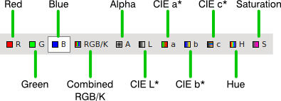
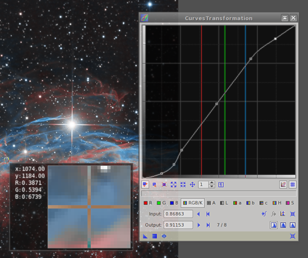
The component selection buttons allow you to select one of the 11 available curves for edition. Each curve is applied to either a nominal channel of an RGB color or grayscale image, or to a dynamically generated image component, as described below.

Red Channel (R)

Applied to the red channel. The red channel is the first nominal channel in RGB color images.

Green Channel (G)

Applied to the green channel. The green channel is the second nominal channel in RGB color images.

Blue Channel (B)

Applied to the blue channel. The blue channel is the third nominal channel in RGB color images.

Combined RGB/Gray (RGB/K)

Applied to the red, green and blue nominal channels of RGB color images, and to the gray nominal channel of monochrome grayscale images.

Alpha Channel (A)

Applied to the active alpha channel. The active alpha channel, when it exists, defines image transparency in PixInsight, and is always the first channel after the nominal channels: either the fourth channel in RGB color images, or the second channel in grayscale images.

Luminance Component (L)

Applied to the dynamically generated CIE L* component of RGB color images. The CIE L* component is computed from the RGB components by means of a RGB to CIE L*a*b* conversion, the curve transformation is applied by interpolation, and the transformed L* component is used to perform the inverse CIE L*a*b* to RGB conversion.

CIE a* Component (a)

Applied to the dynamically generated CIE a* component of RGB color images. The CIE a* component is computed from the RGB components by means of a RGB to CIE L*a*b* conversion, the curve transformation is applied by interpolation, and the transformed a* component is used to perform the inverse CIE L*a*b* to RGB conversion. The CIE a* chrominance component corresponds to the red/green ratio.

CIE b* Component (b)

Applied to the dynamically generated CIE b* component of RGB color images. The CIE b* component is computed from the RGB components by means of a RGB to CIE L*a*b* conversion, the curve transformation is applied by interpolation, and the transformed b* component is used to perform the inverse CIE L*a*b* to RGB conversion. The CIE b* chrominance component corresponds to the blue/yellow ratio.

CIE c* Component (c)

Applied to the dynamically generated CIE c* component of RGB color images. The CIE c* component is computed from the RGB components by means of a RGB to CIE L*c*h* conversion, the curve transformation is applied by interpolation, and the transformed c* component is used to perform the inverse CIE L*c*h* to RGB conversion. The CIE c* chrominance component, or colorfulness, defines color saturation as the distance of a color to the origin of the three-dimensional color space.

Hue Component (H)

Applied to the dynamically generated H (hue) component in the HSV color ordering system. The H component is computed from the RGB components by means of a RGB to HSV conversion, the curve transformation is applied by interpolation, and the transformed H component is used to perform the inverse HSV to RGB conversion. The H component defines color hue as a hue angle from 0 to 360 degrees. However, in PixInsight hue angles are always represented in the normalized [0,1[ range (note the right-open interval), where 1 corresponds to 360 degrees.

Saturation Component (S)

Applied to the dynamically generated S (saturation) component in a special HSVL* color space. The input RGB components are used to perform two conversions, one to the CIE L*a*b* space and another to the HSV space. The curve transformation is applied by interpolation to the H component, and the transformed H component is used to perform the inverse HSV to RGB conversion. The resulting RGB components are transformed to the CIE L*a*b* space, then the new L* component is discarded and replaced with the original one (the original chrominance componets a* and b* are discarded). Finally, a CIE L*a*b* to RGB conversion is performed to yield the final result. This procedure allows, within reasonable limits, for very controllable and smooth color saturation transformations with full preservation of the luminance and no hue changes.

Note that all luminance/chrominance separations are always performed in the RGB working space of the target image. For grayscale images, only the combined RGB/K curve is available; other curves, if defined, are simply ignored for grayscale images.

Point Editing and Navigation

Input

This edit control allows you to manually enter the X (horizontal) coordinate of the current curve point. The X axis corresponds to the input values of the pixel intensity transformation.

Output

Allows you to manually enter the Y (vertical) coordinate of the current curve point. The Y axis corresponds to the output values of the pixel intensity transformation.

Point Navigation Buttons

This is a group of four tool buttons that allow you to select, respectively, the previous curve point, the next point, the first point, and the last curve point.

The one-based index of the current curve point is always shown in the format index/n, where n ≥ 2 is the total number of points in the current curve.

Curve Interpolation

Akima Subspline Interpolation

Select this option to enable Akima subspline interpolation ^[1] for the current curve. This interpolation algorithm has the advantage that when you move a curve point, only its adjacent curve segment(s) is(are) altered, while the rest of the curve remains unchanged. In addition, the PixInsight/PCL implementation ^[2] of Akima subspline interpolation allows defining corner points to connect straight line segments with smoothly curved segments, which provides a great degree of flexibility for manual editing of complex curves. Note that Akima subspline interpolation requires four or more points; when less than four curve points are defined, cubic spline interpolation is automatically used instead. Akima subspline is the default interpolation for CurvesTransformation.

Cubic Spline Interpolation

The cubic spline interpolation algorithm ^[3] ensures continuity of the second derivative for the whole curve. This has the advantage that the resulting curve is always guaranteed to be as smooth as possible, but has the disadvantage that wild oscillations can easily occur between nearby curve points. When oscillations happen, additional points are required to fix them, which sometimes can be difficult to define. In addition, cubic spline interpolation cannot generate straight segments between non-collinear curve points, as a corner point would violate the second derivative continuity constraint.

Linear Interpolation

When linear interpolation is selected, you actually get no curve at all, but an approximation made of straight line segments connecting each pair of adjacent points, or a stroked curve approximation. This mode should normally be avoided since it can generate discontinuities that generally are not desirable. It can be useful only in special cases where jump discontinuities are necessary to reproduce specific image transformations.

Miscellaneous Functions

Store Curve

Click this tool button to store a copy of the current curve. The stored curve can be retrieved later during the current PixInsight session (with the Restore Curve button, see below), but it won't be stored persistently when you exit the PixInsight Core application.

Restore Curve

Click this button to restore a previously stored curve. When you restore a curve, it replaces the current curve —and be careful when doing so, as this operation cannot be undone. Storing/restoring curves is useful to transfer curves among different channels and components.

Invert Curve

Clicking this button will replace the current curve with its symmetric with respect to the horizontal line from {0,0.5} to {1,0.5}. The result of this operation is a new curve that applies the inverse transformation of the original curve. In other words, if C and C' are a curve and its inverse, the we have: ~C(I) = C'(I), where ~ symbolizes the pixel inversion operation.

Reset Curve

This will replace all curve points by two points located at {0,0} and {1,1}, defining an identity transformation (a straight line with slope of 45 degrees). This operation cannot be undone.

Pixel Readouts

The PixInsight Core application generates pixel readouts when you click on an image in readout mode, which is the default working mode for all images (you know the readout mode is active because the image cursor is a simple crosshair). Pixel readouts are sampled pixel values at the current cursor coordinates, and their generation is controlled through a set of readout options that you can define with the ReadoutOptions tool. Pixel readouts are broadcasted to all process interfaces that can receive them. CurvesTransformation is one of those tools.

Figure 1

The CurvesTransformation tool receiving pixel readouts from a RGB color image.

When CurvesTransformation receives pixel readouts, it represents the readout sample values on its curve graph as vertical lines. Each line is plotted at a constant X coordinate equal to the corresponding readout value in the normalized [0,1] range, with a color representative of the sampled image channel or dynamically computed component, depending on the currently selected component. Note that readout lines are plotted for all of the 11 channels and components available.

References

[1] Hiroshi Akima, A new method of interpolation and smooth curve fitting based on local procedures, Journal of the ACM, Vol. 17, No. 4, October 1970, pp. 589-602.
[2] G. Engeln-Mullges and F. Uhlig, Numerical Algorithms with C, Springer, 1996, Section 13.1.
[3] William H. Press et al., Numerical Recipes in C: The Art of Scientific Computing, 2nd Ed., Cambridge University Press, 1992, Section 3.3.
Related Tools
HistogramTransformation, ColorSaturation, RGBWorkingSpace