|
Some Pixel Math Examples |
|
|
|
|
||||||||||||||
|
|
||||||||||||||
|
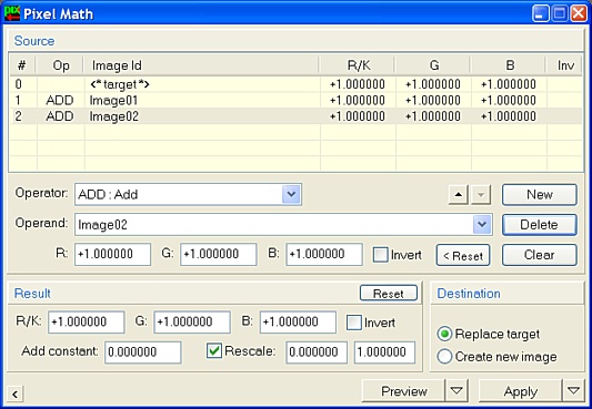
Let's say that you've got three astrophotos of the same subject. You've already registered them so they can be perfectly stacked. The next step will be to integrate them into a single image with improved signal-to-noise ratio. The most well-known method of image integration —and probably the best one, too— is a straight averaging of the whole set of images. Assuming that your images are open in PixInsight and their identifiers are Image01, Image02 and Image03, respectively, the averaging could be easily done with PixelMath, as follows:
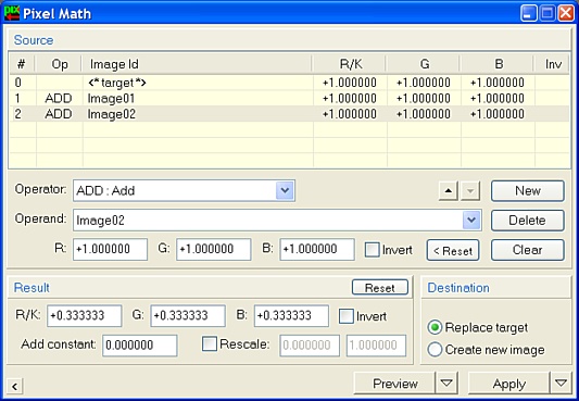
Just apply the above PixelMath process instance to Image03, and job done. PixelMath will add up the three images, which might cause saturation if the dynamic range upper limit is exceeded. However, since rescaling to the normalized [0,1] range has been selected, all data from the three images will be kept in the final result, and no saturation —other than already saturated original pixels— will happen. Because the "Replace target" destination option has been selected, the resulting image will replace your Image03 original. To avoid that, select the "Create new image" destination option. The same thing could be done with:
which instead of relying on the rescaling feature, divides the result by the number of averaged images (3 in the example). Rescaling is somewhat more accurate because it doesn't require entering numerical constants literally.
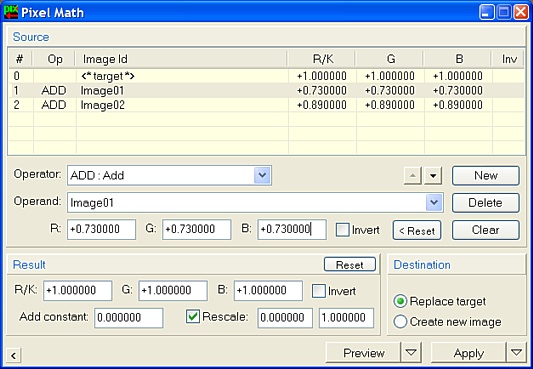
Suppose the same example as before, but the three images haven't been equally exposed —note that this may be due not only to different exposure times, but also to a wide variety of environmental and instrumental factors. Also note that with film images nonlinear film response must be taken into account. When facing differently exposed images, straight averaging is not a correct procedure, since it gives the same statistical weight to all of the signals in the final result, when actually there are signals with different relative strengths. To properly integrate images of different relative exposures, corrective coefficients, or weights, must be applied. Actual coefficient values should be derived from plausible evaluation methods, as densitometric measurements on film originals, or equivalent procedures on digital images. Imagine that, after incredible effort, you've managed to find the magic numbers. The best way to implement a weighted averaging integration with PixelMath might look like this:
Note the coefficients applied to the three color channels of each operand image. The example above assumes that weights have been determined relative to the target image. In addition, it also assumes that different relative exposure times affect equally to the three color channels. Shouldn't be that the case, different weights should be used for each color channel of each operand image. Perhaps the simplest way to apply color corrections to images is to multiply each color channel by an appropriate constant value. This is a linear color correction because it affects equally to all pixels in a color channel, despite their brightness. We think the best way to do this is by using PixelMath:
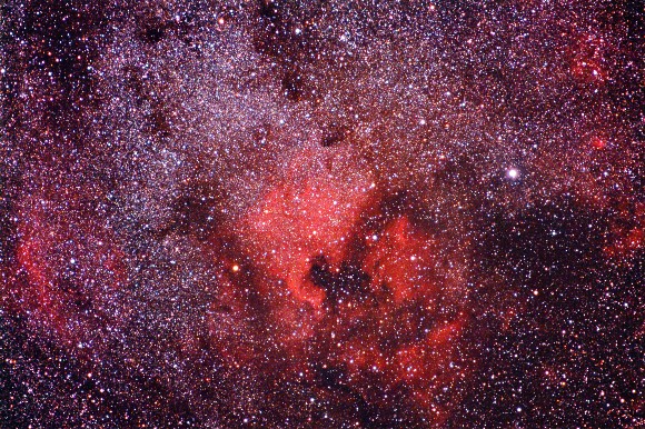
Note the correction coefficients used for red and blue in the result parameters. Since the coefficient for the green channel is exactly one, green is not being altered. Actually, the red and blue corrections are being applied relative to green. In the example above, it is very important to point out that the Rescale result option must not be used. If rescaling is applied, then the process has no effect at all (except a very slight degradation due to round-off error). This is because after multiplication by the specified corrective constant, rescaling forces each channel to occupy the whole dynamic range again, which recovers the original histogram. How about playing with two really different images?
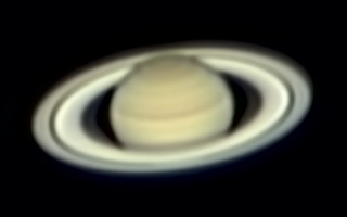
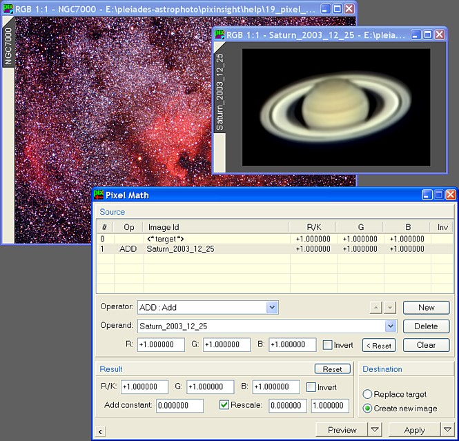
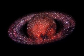
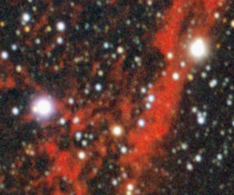
You can save the above images to your hard disk and repeat the examples below; it may be a good way to experiment with PixelMath by yourself. Let's go "artistic" now and combine these two with PixelMath. The images have very different sizes, but you know this is no problem with PixelMath. When needed, operand images are resampled automatically on the fly to match target dimensions. The first thing we'll try is adding both images. This is the setup:
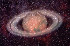
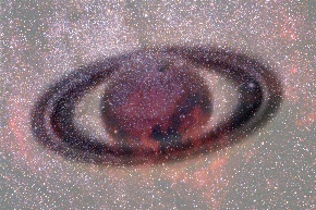
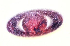
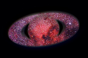
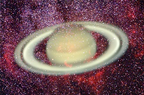
Note the active Rescale option, the ADD operator, and the Saturn image selected as an operand. Naturally, the target image will be NGC7000. Of course the whole set of available operators can be used. This is a little gallery obtained with different operators, applying PixelMath to the NGC7000 image:
More fancy things can be obtained by using inversion for target and/or operand images, as well as for the result. The saturn image can also be applied more than once. Have fun. In his book Photoshop for Astrophotographers, Jerry Lodriguss describes an interesting method of image enhancement based on the screen combine mode of Adobe® Photoshop®. Here we start by defining the screen operation. If F and G are two images, then we have:
where ~ denotes inversion:
This can be very easily implemented in PixInsight with the PixelMath process. Jerry Lodriguss' SMI method consists of the following steps in Adobe® Photoshop®:
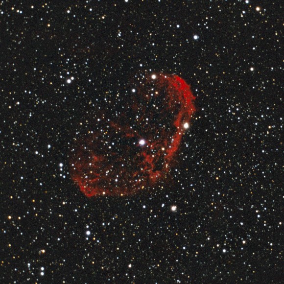
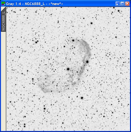
Let's put an example of practical SMI processing in PixInsight. This is the original image:
The image has already been processed in PixInsight Standard 1.0 beta build 129. Four originals were equalized in brightness and color balance, registered, and integrated by averaging. A synthetic background model was generated and subtracted for vignetting correction. Finally, a curves transform was used to achieve neutral background. No further enhancement was done to reveal faint nebular regions and details. The original image is 2048×2048 pixels. Our goal here is trying to enhance this image by the SMI method.
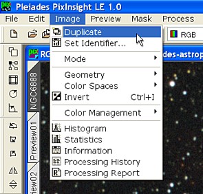
To duplicate the image, the main menu option was used:
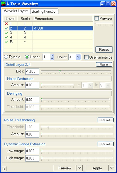
Unfortunately, PixInsight LE does not include the Convolution process that has been implemented in the standard version. Convolution is the natural choice to blur images by Gaussian filtering. However, wavelets processing can be applied in PixInsight LE with the same purpose. This is done very easily by disabling or weakening some small-scale wavelet layers. In our example, the following ATrousWaveletTransform instance did a pretty good blurring job. Here is a screenshot of the À Trous Wavelets window showing relevant parameters:
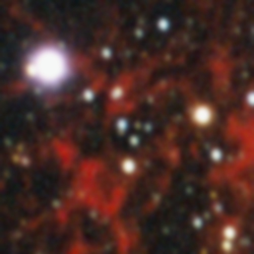
The default 3x3 Linear wavelet scaling function was used. Note the disabled Use luminance option to act on both luminance and chrominance. By disabling the first wavelet layer and applying a negative bias to the second layer, high-frequency spatial components have been conveniently removed from the image. Below is a mouseover comparison between the original and blurred images. Note that a relatively slight blurring effect has been applied. If you want to play with different softening amounts, take into account that the SMI method is quite sensitive in this regard.
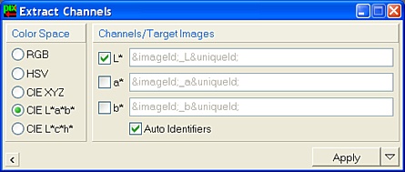
The Extract Channels processing window is used as shown below:
Note the CIE L*a*b* color space and the disabled a* and b* channels. Applying this process to the original image, we get the luminance in a new image window. After using (Ctrl-I), this is the result:
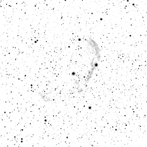
The original SMI method uses just this mask. However, we can improve the SMI process by clipping the highlights of the inverse luminance mask with a simple histograms transform. After this adjustment, the mask used in our example is shown below.
In addition to protect stars from excessive bloating, this mask will also help preventing oversaturation of the brightest nebular regions. If more protection is needed for particular areas, the mask can be further modified with curves and other usual techniques, or even it can be combined with other masks.
For the mask image to act as such, it must be selected as the active mask for the original. Having the original image selected, this is done with the (Ctrl-M) main menu option, or by clicking the corresponding tool button. Unless you have changed this behavior in global preferences, every time a mask is selected PixInsight shows it over the masked image to inform you of protected areas. You'll probably have to select to hide the mask.
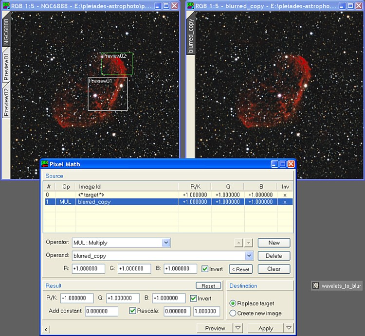
The figure above shows Pixel Math ready to perform the SMI enhancement. We recall here the Screen operation formula for two images F and G:
and recall also that the tilde '~' symbol denotes inversion of pixel values: ~x = 1 – x. Three inversion operations are required for Screen, as you see in the expression above. See them also on the figure. The Invert option is active for the target image, for the ''blurred_copy" operand image, and also for the result. Finally, the multiplication operator has been selected for the operand. The Rescale option isn't actually necessary here, but it will allow for a better dynamic range usage. After applying the above PixelMath instance to the NGC6888 image, this is the result: The SMI technique enhances faint detail without bloating star images. Background noise is also reduced because a low-pass filtered version of the image is combined with the original. By adjusting the amount of blurring and carefully altering the mask, very good results can be obtained for many deep-sky astrophotos. As Jerry Lodriguss says in his book: "This is as close as it gets to having something for nothing". |