|
The HistogramsTransform Process
Histograms are dynamic objects in PixInsight. They are calculated and generated automatically when necessary. Any view of an image window can be selected on the Histograms window to inspect and manipulate its histogram functions. When a view is selected this way, its histograms are immediately calculated if they don't already exist. When the selected view is modified in any way that modifies its pixel contents, its histograms are automatically recalculated and the Histograms window is updated accordingly.
Histograms are internally generated with 16-bit resolution (65536 levels). However, they can be displayed and inspected with interpolated resolutions varying in the range from 100 levels to the full 16-bit precision, including the standard 8-bit (256 levels) 10-bit (1024 levels) and 12-bit (4096) binary resolutions. This allows for precise adaptation of the histogram graphics and manipulation tools to the specific contents of each image.
HistogramsTransform implements a direct pixel manipulation defined by a set of specific parameters:
- Shadows Clipping
- Highlights Clipping
- Midtones Balance
- Dynamic Range Expansion Lower Bound
- Dynamic Range Expansion Upper Bound
HistogramsTransform parameters are real numbers in the normalized dynamic range: from 0 (no signal, black) to 1 (full signal, white). This gives full independence on specific bit depths.
For grayscale images, a unique set of parameters is used. For RGB color images, three independent sets of parameters are applicable.
Clipping Parameters
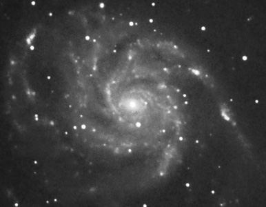
Clipping parameters define a relative reduction of the dynamic range usage in the image. Any pixel below the shadows clipping bound will be assigned a zero (black) value, while pixels above highlights clipping will be set to one (white). Remaining pixel values between both clipping bounds will be proportionally rescaled to extend over the full normalized dynamic range. Figure 1 shows how clipping parameters work for a typical astronomical image.
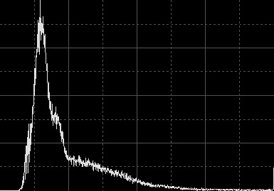 |
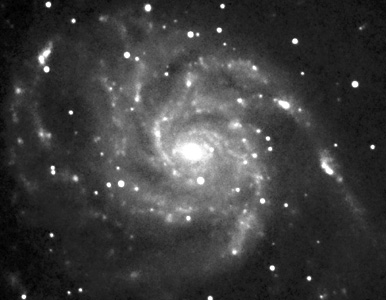
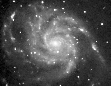
Figure 1a — The original image and its histogram. The central region of the M101 spiral galaxy in Ursa Major.
Note the unused portion of dinamyc range at the shadows end (left) of the histogram. This denotes a bright sky background.
Also note the small vertical peak at the highlights end (right) of the histogram. This corresponds to white pixels accumulated on saturated stellar objects.
|
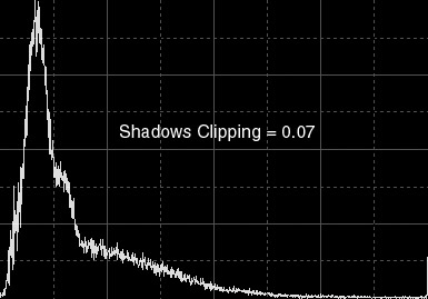 |
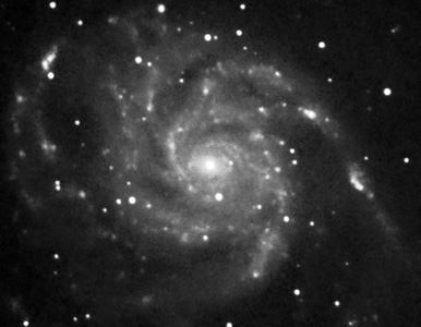
Figure 1b — Clipping at the shadows end. The image and its resulting histogram after applying a histogram transform consisting on a single shadows clipping value of 0.07
The applied transform virtually has not clipped (set to black) any pixels. Now pixel values in the image have been rescaled for a better usage of the whole dynamic range.
As a result of this transform, the background is darker and the overall contrast is higher without highlights saturation.
|
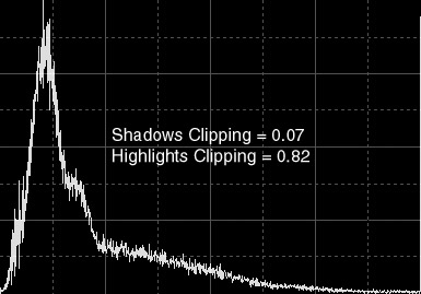 |
Figure 1c — Clipping at both shadows and highlights. The image and its resulting histogram after applying a histogram transform defined by a shadows clipping value of 0.07 and a highlights clipping value of 0.82 to the original.
While the shadows clipping value used is the same as above, so no pixels have been clipped in the shadows of the image, highlights clipping has been severe and shows itself as a prominent vertical peak at the highlights end of the resulting histogram.
Sky background remains correct, as above, but now many bright features are saturated, including the galaxy core and most stellar objects. The applied transform is quite incorrect for this image since it has resulted in a severe information loss.
|
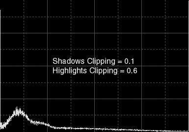 |
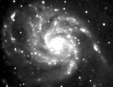
Figure 1d — An example of disastrous histogram transform. Beginners do things like this sometimes. This is what happens when a shadows clipping of 0.10 and a highlights clipping of 0.60 are applied to the original image.
Both clipping values are by far excessive, as denoted by the big vertical peaks at both ends of the histogram. Data loss is extremely severe in this example.
|
Midtones Balance
The midtones balance parameter of HistogramsTransform can take values in the entire normalized dynamic range (from 0 to 1). It defines a midtones transfer function (MTF) that is applied to every pixel after clipping has taken place. A midtones balance value of 0.5 defines a linear identity function, i.e. no change occurs. Values below 0.5 increase midtones, while values above 0.5 darken midtones in the image. In Figure 2 some MTFs are exemplified.
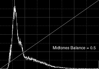 |
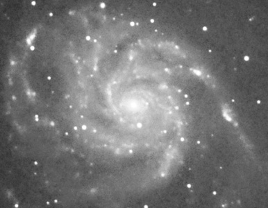
Figure 2a — The original image and its histogram. An identity midtones transfer function (MTF) has been drawn over the histogram.
|
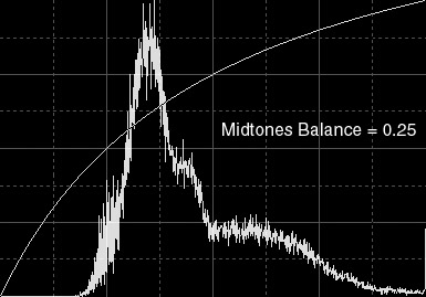 |
Figure 2b — Enhancing Midtones. These are the resulting image and histogram after applying a MTF defined by a 0.25 midtones balance.
Background pixels are now considerably brighter as a result of increased overall brightness. Note how the histogram maximum has been displaced towards the right side, staying now much closer to the center. This says that there are more pixels with midtone (intermediate) values now, as intended with the MTF used, but most of these pixels are located on sky background areas.
|

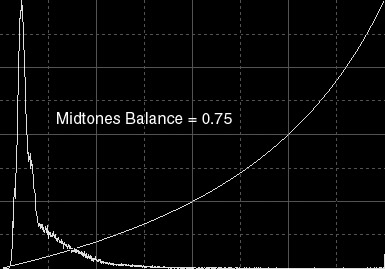 |
Figure 2c — Weakening midtones. These are the resulting image and histogram after applying a MTF defined by a midtones balance value of 0.75.
Contrarily to the above MTF, now the histogram maximum has been displaced to the left (shadows) side, as a result of decreased overall brightness. The background is much (too) darker and there are much more pixels with low values now.
|
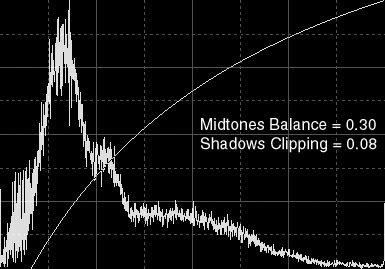 |
Figure 2d — Simultaneous shadows clipping and midtones enhancement. To the left you can see the results of a histogram transform defined by a 0.30 midtones balance value and a 0.08 shadows clipping.
The MTF applied enhances midtones, but it also extends the length of the initial segment of unused dynamic range, as shown by the histogram of Figure 2b.
By specifying a reasonable nonzero value for the shadows clipping parameter, this situation is corrected and the dynamic range usage is significantly improved. Higher midtones show more detail on galaxy arms, but shadows clipping ensures correct background levels and overall contrast.
A vertical peak has arised at the shadows end of the histogram. While this denotes zero-clipped pixels, the amount of clipped pixels is not significant and all of them are background pixels, which are very likely to be noise. The black peak can be easily corrected by a simple noise reduction.
|
Dynamic Range Expansion
The dynamic range expansion lower bound parameter of HistogramsTransform can vary from –10 to 0, while dynamic range expansion upper bound ranges from 1 to 10. These two parameters actually allow expansion of the unused dynamic range at both ends of the histogram. This can be probably better understood as a two-step procedure: first, dynamic range is expanded to occupy the entire interval defined by the lower and upper bound parameters, but actual pixel values are not changed. The second step is to rescale both dynamic range and pixel values back to the normalized [0,1] range. The result of this process is that all pixel data are constrained to a smaller effective interval, and free unused portions appear at the histogram ends. This is used as a previous step for some image processing techniques with the purpose of preserving actual pixel data from losses due to excessive contrast gains.
To illustrate how this actually works, we'll use a new series of examples with the same M101 image, as above. Figure 1a shows the original image and histogram.
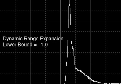 |
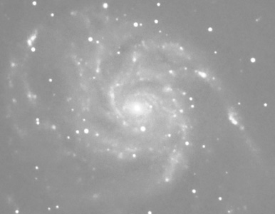
Figure 3a — Dynamic range expansion:
lower bound = –1.
Once rescaled to the normalized [0,1] range, the minimum pixel value is 0.5 in this example, which brightens the entire image uniformly.
|
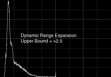 |
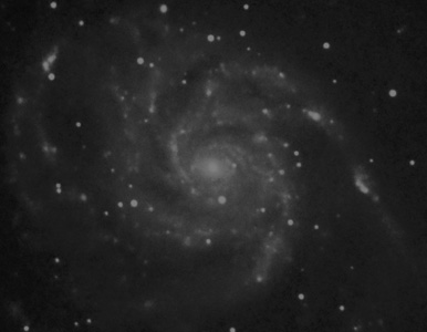
Figure 3b — Dynamic range expansion:
upper bound = +2.
This time standard rescaling imposes a maximum pixel value of 0.5, which in turn darkens the entire image uniformly.
|
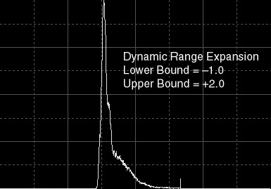 |
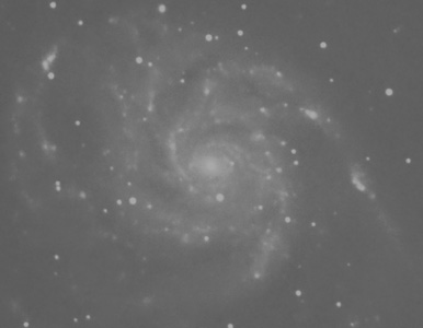
Figure 3c — Dynamic range expansion:
lower bound = –1, upper bound = +2.
After standard rescaling, pixel values are constrained to the 1/3 to 2/3 interval. This causes an overall contrast loss such as the image seems "washed".
|
|